General Principles of Doppler Imaging

Efforts to map the spot structure on stars, either in the form of cool starspots or in the form of the pattern of distribution of anomalous abundances for Ap stars, were frustrated because of the high precision of the spectroscopic data needed for the task. Photographic spectra were of poor signal-to-noise but with the advent of digital detectors such as Reticons and CCD arrays, a signal-to-noise level of many hundreds to one could easily be achieved in observed stellar spectra. Thus, with high dispersion and high resolution spectrographs, the changing line profile shapes of spectra could be monitored accurately throughout the rotation period of the stars whose variability was due to surface features that were moving across the visible face of stars as they rotated. At about the same time that electronic detectors became available, abundant computing power (along with excellent display features) also became available. With excellent line profiles and good computing power the data in the spectral profiles could be inverted to form an image of the star using a technique called Doppler Imaging.

The General Principles of Doppler Imaging

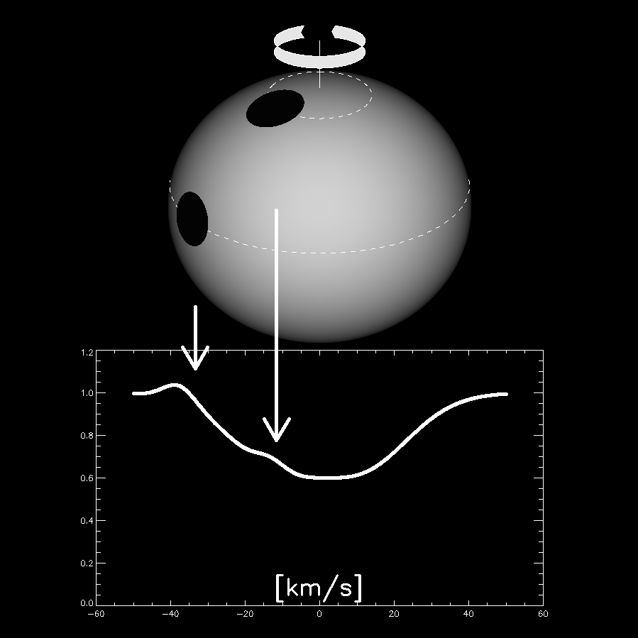
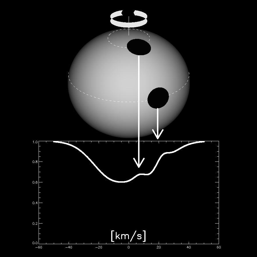
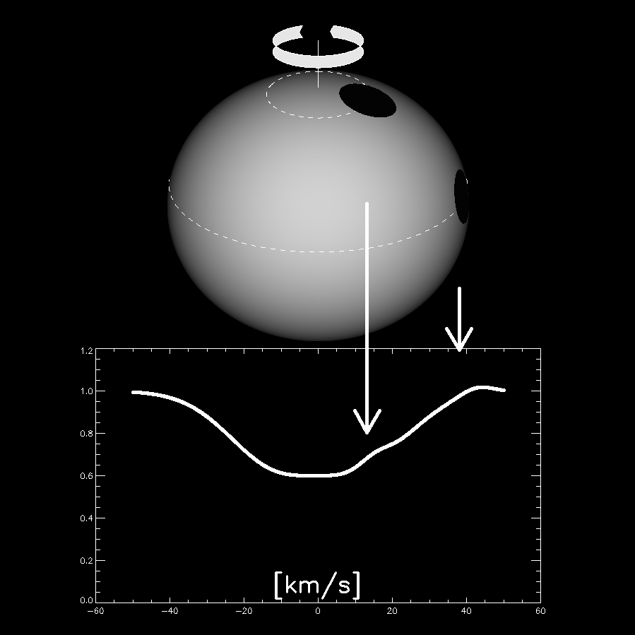
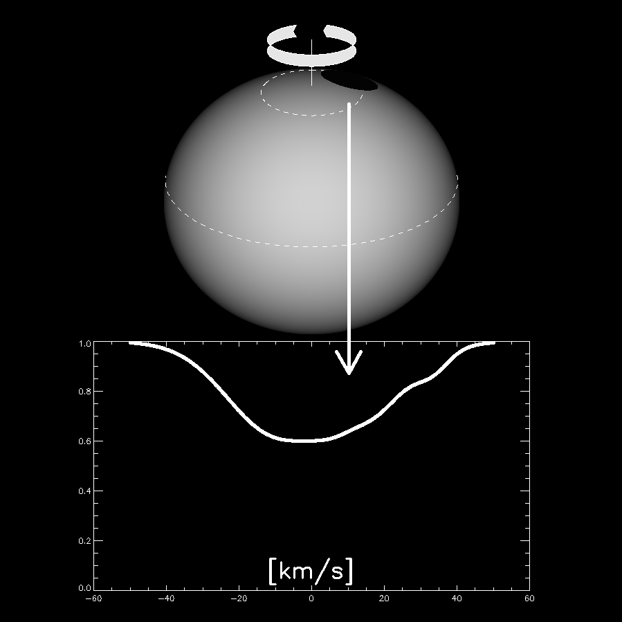
The inversion process to produce images of surface features on spherical stars is straightforward in concept. To understand the essentials, first think of a star that might have a single small cool starspot on its surface. If the star is rotating quickly enough that the rotational broadening of the profile is significantly larger than the local line width on the stellar surface, the observed stellar line will show a”bump” that will move across the line profile as the star rotates, moving from the blue wing to the red. Small  spots on the surface of the star are mapped onto the stellar line profile at any given phase such that the forward calculation gives a well defined location for the “bump” in the profile. The reverse calculation of mapping the “bump” onto the star’s surface gives a locus of points on the stellar surface that could be occupied by the spot source. This indeterminacy in spot mapping is resolved by taking multiple observations at reasonably well spaced phases.

As can be seen from image1,  image 2, image 3 and image 4, the phase when a profile “bump” crosses the line centre gives the longitude of the spot and the latitude is logically deduced from the temporal behaviour of the “bump”. Low latitude spots would give a profile “bump” that is evident for half a rotational phase and that moves from the extreme blue to the extreme red across the profile. Higher latitude spots display a “bump” that is evident for a much larger fraction of the rotational phase and that actually moves from red to blue briefly, after first coming into view over the pole of the star, before reverting to the more normal direct blue to red motion. The excursion of the “bump” in wavelength is much smaller for these high latitude spots. For cool stars where the surface features are cool spots locally radiating less light in the continuum the “bump” is like an emission peak in the line profile.  For those of us who also work with Ap stars where the surface anomalies are usually spots of enhanced abundance, the “bump” is a small valley of greater line depth.

You can see a video of the behavior of spots at three different latitudes here.

In all cases, the surface features are much more complicated than a simple circular spot so the mapping process for real stars is, of course, more complex than the preceding paragraph would suggest

The mathematical process of Doppler imaging is essentially always a matter of creating an error function that represents the degree to which the predicted spectrum from a current trial image of a star (the forward calculation) differs from the observed spectrum. Then the trial image is iteratively adjusted to reduce the error function to a minimum consistent with the error of the observations. The trial image starts as a surface with uniform temperature and a gradiant is created from the error function that gives the extent to which the error would be reduced by altering the temperature at each surface point. A penalty function keeps the alteration of the temperature from exceeding that which is consistent with the signal-to-noise in the data. A forward calculation using the improved trial image is done including all the physics of spectrum line formation and the geometry of rotation to find the new error between observed and trial spectrum. This is followed by another gradient to determine what adjustments should be made at each point on the trial star’s surface.